Lecture 4: A Simple Economic Model |
||||||||||||||||||||||||||||||||||||||||||||||||||||
|
The last lecture discussed data, not how the economy works. This lecture begins with the task of developing a simple economic model. |
||||||||||||||||||||||||||||||||||||||||||||||||||||
The Basic Model |
||||||||||||||||||||||||||||||||||||||||||||||||||||
|
This basic model that we start to develop in this lecture and finish in the next few lectures will used throughout the rest of the class. It consists of four sectors and the rest of the class uses one or more of these parts when discussing an issue. |
||||||||||||||||||||||||||||||||||||||||||||||||||||
The Robinson Crusoe Economy |
||||||||||||||||||||||||||||||||||||||||||||||||||||
|
We will begin by thinking out the problems faced by a single individual living on a deserted island. Economists call this the Robinson Crusoe Model, after the hero of Daniel Defoe's famous novel. As you recall, Crusoe was shipwrecked on a deserted island. Initially alone on the island, Crusoe had to fend for himself. While he managed to retrieve some supplies from the ship, he basically depended on what he produced, either by picking berries from trees, setting traps, building some primitive housing to protect himself from the storms, etc. |
||||||||||||||||||||||||||||||||||||||||||||||||||||
The Production Function |
||||||||||||||||||||||||||||||||||||||||||||||||||||
|
Of course, how well Crusoe lived depended on just how hard he worked. If he just spent his time sitting on the beach (hopefully under a shade tree) he would starve. His well being depended on just how many hours a day he spent working. |
||||||||||||||||||||||||||||||||||||||||||||||||||||
|
To an economist, that means Crusoe had a production function describing the relation between how hard he worked and how many berries he was able to collect a day. The harder he worked, the more berries he was able to collect, the better the house he was able to build, etc. There are several ways of describing the production function. We could do so either via a table describing the number of berries he collected a day, which would be Crusoe's GDP, or we could describe it with the aid of a simple graph. To be complete, we will do so both ways, for we shall learn something from both. |
||||||||||||||||||||||||||||||||||||||||||||||||||||
|
Table 4-1 shows a possible production function for Crusoe, showing how the number of berries depends on the hours of work each day. |
||||||||||||||||||||||||||||||||||||||||||||||||||||
|
||||||||||||||||||||||||||||||||||||||||||||||||||||
|
This table has four columns. |
||||||||||||||||||||||||||||||||||||||||||||||||||||
|
· Column one lists the number of hours Crusoe could work each day. |
||||||||||||||||||||||||||||||||||||||||||||||||||||
|
· Column two gives the number of berries he would collect. As you will note, it is obvious that Crusoe's GDP should be measured in terms of berries per day. This column gives his total product as a function of the number of hours worked. |
||||||||||||||||||||||||||||||||||||||||||||||||||||
|
· Column three provides his average product, or berries per hour. |
||||||||||||||||||||||||||||||||||||||||||||||||||||
|
· Column four gives the marginal product, the number of additional berries from an additional hour of work. As discussed in the first lecture when we talked about Malthus, each additional hour of labor supplied produces less output than the previous hour of labor. |
||||||||||||||||||||||||||||||||||||||||||||||||||||
|
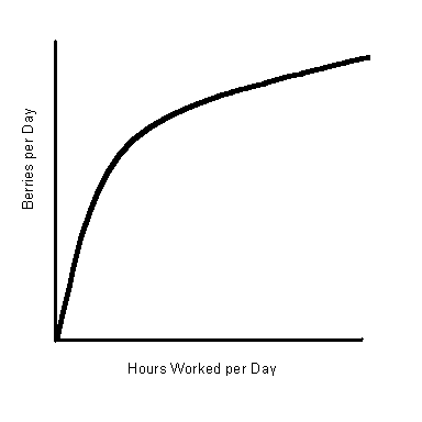
We can also put the production function as a graph. Figure 4-1 shows what the Crusoe production function would look like graphically. |
||||||||||||||||||||||||||||||||||||||||||||||||||||
|
||||||||||||||||||||||||||||||||||||||||||||||||||||
|
Note that this graphical representation, like the tabular representation, has the property of diminishing returns. Whenever Crusoe increases his hours of work, he increases the number of berries he picks, but not in proportion. For example, when he increase his hours worked from three per day to four per day, a 1/3 percent increase, the number of berries rises from 3,000 to 3,500 per day, only a 1/6 increase. Several factors obviously contribute to diminishing returns to proportion. Among others, he gets tired and he has to reach further to pick additional berries. |
||||||||||||||||||||||||||||||||||||||||||||||||||||
The Production Possibilities Frontier |
||||||||||||||||||||||||||||||||||||||||||||||||||||
|
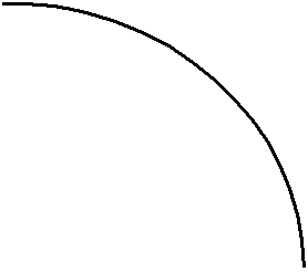
Another way of putting Crusoe's choice is in terms of a production possibilities frontier, representing the choices between leisure time and berries. If he chooses not to work at all, he will get 24 hours a day of leisure, but zero berries. The harder he works, the more berries but the fewer hours of leisure. |
||||||||||||||||||||||||||||||||||||||||||||||||||||
|
||||||||||||||||||||||||||||||||||||||||||||||||||||
|
Figure 4-2 shows the production possibilities frontier. As you will note, the production possibilities frontier and the production function give the same information, but just expressed in different ways. |
||||||||||||||||||||||||||||||||||||||||||||||||||||
|
How much time will Crusoe spend each day picking berries? We do not have enough information to tell. It depends on Crusoe's preferences for food and free time. That Crusoe must decide how much time to spend working should serve as a reminder that his well being depends, not only on his GDP, the number of berries he collects, but also on other factors such as the amount of free time he gets. |
||||||||||||||||||||||||||||||||||||||||||||||||||||
Jazzing up the Model |
||||||||||||||||||||||||||||||||||||||||||||||||||||
|
Crusoe lived a very simple life, but not quite as simple as the one described here. The simple story we are telling here indicates that, each day, Crusoe spent his working hours collecting berries to eat that day. That is, all of his working time was devoted to production for consumption. In fact, Crusoe could do – and did – other things. He spent some time building a shelter, some time exploring the island for better patches of berries, and perhaps building machines to make berry picking easier. The time Crusoe spend each day in those activities was clearly part of his Gross Domestic Product, though it clearly is not consumption. In short, Crusoe could invest. Thus we want to write Crusoe's GDP as |
||||||||||||||||||||||||||||||||||||||||||||||||||||
|
Y = C + I |
||||||||||||||||||||||||||||||||||||||||||||||||||||
|
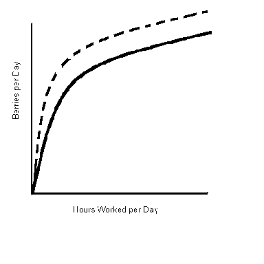
Over time, these investments will shift out Crusoe's production function, as Figure 4-3 illustrates. |
||||||||||||||||||||||||||||||||||||||||||||||||||||
|
Of course, this is not the only thing that can shift Crusoe's production function. A partial list would include: |
||||||||||||||||||||||||||||||||||||||||||||||||||||
|
· Variable weather. Rainy days are not good days for picking berries, and at some times of the year, berries are more plentiful than on other days. |
||||||||||||||||||||||||||||||||||||||||||||||||||||
|
· New discoveries. Crusoe can find new and better ways of picking berries. |
||||||||||||||||||||||||||||||||||||||||||||||||||||
|
One final factor that, while it will not shift the production function, can cause movement along the production function. |
||||||||||||||||||||||||||||||||||||||||||||||||||||
|
· Crusoe was, like most of us, highly motivated some days and inclined to "relax" other days. |
||||||||||||||||||||||||||||||||||||||||||||||||||||
|
|
||||||||||||||||||||||||||||||||||||||||||||||||||||
|
||||||||||||||||||||||||||||||||||||||||||||||||||||
|
A naïve interpretation of these daily fluctuations in the number of berries picked look like business cycles, and, on the days when Crusoe is not working very hard, the naïve interpretation is that he is "unemployed" or at least "underemployed". We know better. Fluctuations in the desire to work and to take leisure as well as climate fluctuations account for these variations. |
||||||||||||||||||||||||||||||||||||||||||||||||||||
|
Nonetheless, some economists do interpret these fluctuations as business cycles, and we will have more to say about them later. |
||||||||||||||||||||||||||||||||||||||||||||||||||||
A Model with Trade |
||||||||||||||||||||||||||||||||||||||||||||||||||||
|
The Robinson Crusoe economy is what economists call an Autarchic Economy. Crusoe produces all he consumes and invests; all that he consumes and invests comes from his own production. |
||||||||||||||||||||||||||||||||||||||||||||||||||||
|
In fact, all real-life economies involve many different people producing many different goods, buying and selling production from each other either by contract or negotiation. That is, people trade with each other, and we want to expand the model to allow for trade. When we do, we will have to account for three more factors in our model: |
||||||||||||||||||||||||||||||||||||||||||||||||||||
|
· Labor Markets |
||||||||||||||||||||||||||||||||||||||||||||||||||||
|
· Money |
||||||||||||||||||||||||||||||||||||||||||||||||||||
|
· Unemployment |
||||||||||||||||||||||||||||||||||||||||||||||||||||
Labor Markets and GDP |
||||||||||||||||||||||||||||||||||||||||||||||||||||
|
Suppose Robinson Crusoe and thousands like him are suddenly transported, perhaps by a transporter vis-a-vis Star Trek, to an island peopled with thousands of individuals much like him. They would quickly discover the advantages of working together, each one producing a different good and then trading the goods with one another. Crusoe might continue to pick berries, while someone else would spend time catching fish, and yet another person might spend time weaving baskets both for the fish and for the berries. A lively market trading fish for berries for baskets would then ensue. Our citizens would have quickly discovered the advantages of specialization, a subject we will return to later in this course. We can all produce more if we specialize in different products. Robinson Crusoe might specialize in picking berries, eating some of the berries he finds, but then trading most of his berries for fish, baskets, and the other goods he wants to consume. |
||||||||||||||||||||||||||||||||||||||||||||||||||||
|
||||||||||||||||||||||||||||||||||||||||||||||||||||
|
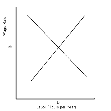
There is an important issue here. Crusoe is not selling berries, but his time for finding berries. So are the other producers. In effect, we have a labor market, in which people buy and sell labor services. Some people will form business firms and hire workers, and other people will decide to work for those firms. In short, we will now have a supply and demand for labor. Figure 4-4 illustrates the demand and supply for labor. To make the discussion simple we will not worry about the long run and short run labor supply curves here, though we will return to that issue later. |
||||||||||||||||||||||||||||||||||||||||||||||||||||
|
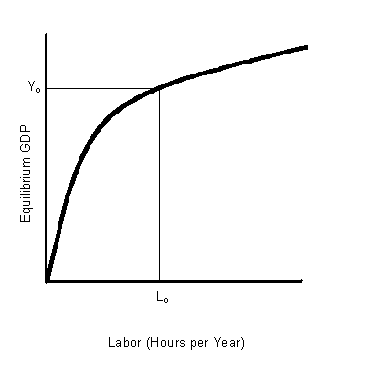
Moreover, just as Robinson Crusoe had a production function so too does the economy have a production function. Holding capital and technology constant, as we did in the case of Crusoe, our production function gives output as a function of the number of hours worked each year. In turn, that determines total GDP. Figure 4-5 illustrates the determination of the total level of output. |
||||||||||||||||||||||||||||||||||||||||||||||||||||
|
||||||||||||||||||||||||||||||||||||||||||||||||||||
Warning required by the Economist-General: |
||||||||||||||||||||||||||||||||||||||||||||||||||||
|
· This lecture introduces the model we will be using throughout this course. It is a simple one, involving some important simplifying assumptions. |
||||||||||||||||||||||||||||||||||||||||||||||||||||
|
· When people are working together in an economy, common sense suggests that labor markets do arise. Individuals work for pay, either as employees of a firm or as self-employed workers. The process by which labor markets arise is more complicated than we suggest here. At the same time, labor markets do not necessarily work as smoothly or as effortlessly as this lecture suggests. We will have a lot more to say about that later. |
||||||||||||||||||||||||||||||||||||||||||||||||||||
|
· Finally, we assume that all workers are identical, so we can talk about the demand and supply for workers, as opposed to the demand and supply of (say) bricklayers and bakers. This simplifying assumption is very much in the spirit of macroeconomics and, as we shall see later, is one of the reasons why labor markets do not work as smoothly or as effortlessly as this lecture suggests. |
||||||||||||||||||||||||||||||||||||||||||||||||||||
Money |
||||||||||||||||||||||||||||||||||||||||||||||||||||
|
While the important idea of this model, is that, as in a real economy, people are exchanging services with each other, they do not do so directly. If we really insisted on direct exchanges, the effort would be maddening. Instead, we buy and sell our services for money. The bricklayer is paid in dollars, euros, or yen, depending on the country, and then uses the money to purchase other products such as berries or bread. That is, while the exchange takes place in terms of pictures of George Washington or the favorite national icon, the real exchange is bricklaying for bread and berries. However, it is much more convenient to do so via money. We only need look at the disorder in countries where their local money does not work to see the importance of using money as the medium of exchange. |
||||||||||||||||||||||||||||||||||||||||||||||||||||
|
That means we want to look at how our monetary system works, and in particular, we want to look at some essential variables. |
||||||||||||||||||||||||||||||||||||||||||||||||||||
|
· The nominal money supply (Ms) measures the supply of money in the economy in terms of dollars or some other national unit. For example, by one measure, the nominal money supply of the United States is about $1.3 trillion. That is there are 1.3 trillion pictures of George or the equivalent (a picture of Abraham Lincoln is the equivalent of five pictures of George). |
||||||||||||||||||||||||||||||||||||||||||||||||||||
|
· The velocity of money (V) measures the average number of times that each dollar is used each year. The intuitive idea behind this equation is a simple one. Money is the lubricant that keeps the economy functioning, and a certain amount of money is required for each dollar of GDP. |
||||||||||||||||||||||||||||||||||||||||||||||||||||
|
If we multiple the Money Supply by Velocity we get the total amount of spending that occurs in an economy in a year. Total dollars spent in a year is just another way to say Nominal GDP. If you remember from a previous lecture Nominal GDP is composed of two parts: Real GDP (y) and the Price Level (P). Therefore, |
||||||||||||||||||||||||||||||||||||||||||||||||||||
|
|
||||||||||||||||||||||||||||||||||||||||||||||||||||
Money Supply times Velocity = Price level times Real GDP |
||||||||||||||||||||||||||||||||||||||||||||||||||||
|
|
||||||||||||||||||||||||||||||||||||||||||||||||||||
|
Put into symbols: Ms V = P y |
||||||||||||||||||||||||||||||||||||||||||||||||||||
|
|
||||||||||||||||||||||||||||||||||||||||||||||||||||
|
This equation is called: The Equation of Exchange |
||||||||||||||||||||||||||||||||||||||||||||||||||||
|
|
||||||||||||||||||||||||||||||||||||||||||||||||||||
|
Look at the variables in this equation. Real GDP is determined by the number of people working (see figure 4-5) and the money supply is determined by the government. If velocity is set by factors such as how often we are paid, then the price level must be determined by the equation of exchange. That is |
||||||||||||||||||||||||||||||||||||||||||||||||||||
P = MV/y |
||||||||||||||||||||||||||||||||||||||||||||||||||||
Warning required by the Economist-General: |
||||||||||||||||||||||||||||||||||||||||||||||||||||
|
· The equation of exchange is one of the most important equations in macroeconomics. We return to this equation repeatedly throughout this course. For the moment, Velocity is a constant. In a later lecture, we will discuss some of the factors that actually determine velocity. |
||||||||||||||||||||||||||||||||||||||||||||||||||||
|
|
||||||||||||||||||||||||||||||||||||||||||||||||||||
|
This model tells us something important about how the economy works. Suppose the money supply is initially $1,000 and the government raises it permanently to $2,000. We know that y, real GDP is determined by the supply and demand for workers and the production function. If M doubles, then the right hand side of this equation doubles, and, in turn, this means that P must double. That is, changes in the price level come about because of changes in the money supply. |
||||||||||||||||||||||||||||||||||||||||||||||||||||
|
We would also expect nominal wages, expressed like prices, in terms of pictures of George Washington to double as well. The effect will be to leave real wages unchanged. If the nominal wage rate goes from $6 an hour to $12 an hour while pizzas go from $6 to $12, then one's real wage, one pizza per hour, remains unchanged. |
||||||||||||||||||||||||||||||||||||||||||||||||||||
|
This proposition is sometimes referred to as the neutrality of money. That is, changes in the money supply change the price level, but leave real GDP, real employment and real wage rates unchanged. This is sometimes popularized by saying "money does not matter", but nothing could be further from the truth. Money does not matter. We cannot have a modern economy without money. A more correct statement is that a change in the number of pictures of George does not matter. |
||||||||||||||||||||||||||||||||||||||||||||||||||||
Relation to the Text |
||||||||||||||||||||||||||||||||||||||||||||||||||||
|
Each lecture ends with a section relating it to the text. In some cases, material is omitted, either because the text covers it well enough or because it is not worth learning. In other cases, material is added. Each of these “lectures” will end with a brief note relating the lecture to the text, describing what material is left to the student to learn alone and what material may safely be skipped. |
||||||||||||||||||||||||||||||||||||||||||||||||||||
Which Chapters does this lecture cover? |
||||||||||||||||||||||||||||||||||||||||||||||||||||
|
|
||||||||||||||||||||||||||||||||||||||||||||||||||||
What material is new? |
||||||||||||||||||||||||||||||||||||||||||||||||||||
|
None for this lecture. |
||||||||||||||||||||||||||||||||||||||||||||||||||||
|
©2000 by
Greg Chase and Charles W. Upton. If
you enrolled in Principles of Macroeconomics at Kent State University, you
may print out one copy for use in class.
All other rights are reserved. |
||||||||||||||||||||||||||||||||||||||||||||||||||||
