Lecture 5: Saving and Investment

We showed previously how Crusoe could divide his GDP between consumption and investment by dividing his time between the production of goods he would consume immediately and goods that would yield future benefits. In a modern society, the division is more complicated. We now turn to the subject of what determines the division of GDP between consumption and investment. We will also go beyond Crusoe and include government borrowing and international trade in our discussion.

One thing that makes our task simple is that the resources for investment come from saving. Therefore, rather than talk about how people decide how much to consume, we will talk about how people determine how much to save. Since income after taxes goes for either consumption or saving, it is a matter of twiddle dee or twiddle dum.

Saving and Investment as Different Concepts

Many people confuse the concepts of saving and investment. The differences are important, so we will spend some time on the issue.

Saving takes place when people abstain from consumption, that is, when they consume less than their income. Investment takes place when we purchase new capital equipment or other assets that make for future productivity. Investment does not mean buying stocks or bonds. Here are some important facts:

· For Robinson Cruse, the difference between saving and investment is a distinction without a difference. Since he does all saving and all investment, they are automatically equal. However, for the larger economy, this is not true. Investment funds come either from our own saving or from someone else's saving.

· The motive for saving is one of deferring your consumption to a later day. We save when we consume only part of our income now and save for retirement, a rainy day, putting children through college, the summer home, etc.

· The motive for investment is to make money. Investment takes place when we purchase plants or equipment, which make workers and businesses more productive in the future.

· Ultimately saving and investment must be equal, (subject to a couple of complications that make for nice exam questions). As you will see in a moment, you can think of saving as a supply of funds for investment and investment as a demand for funds. We will later draw supply and demand curves and show how saving and investment are equated.

Table 5-1 Some Examples of Saving and Investment
The Facts	Saving or Investment?
The owner of Miller's Pizzeria has after tax income of $50,000 this year. He spends $40,000 on consumption, and decides to save the rest by investing in a $10,000 certificate of deposit at the 87^th National Bank. This brings his accumulated deposits to $50,000.	$ 10,000 in saving. The word “invest” is misused. The rest of the deposits constitute savings, or cumulative saving.
The owner decides to purchase a new $10,000 pizza oven, paying for it by taking $10,000 out of the savings account at the 87^th National Bank.	Investment.
In the next year, the owner decides to purchase a new, high tech oven for $25,000, paying for it by leaving $5,000 in earnings in the business and taking an additional $20,000 loan from the Bank.	Both. The new oven is an investment of $25,000, and he saved $5,000 this year by not taking part of the money out of the business for spending.

Warning required by the Economist-General:

· Points are deducted on all exams for confusing saving and investment.

Investment

Some Preliminaries on Interest Rates

An understanding of interest rates is important for understanding saving and investment. Put simply, an interest rate is the price of a loan, expressed as a percentage of the amount loaned each year. Thus, if the interest rate is 6%, and you borrow $100, you must pay back $106 at the end of the year. Moreover, when you deposit $10,000 in a certificate of deposit you are effectively making a loan to the bank or other financial institution. The interest rate is the price the bank pays you. In short, interest is either the reward you get for saving or the premium you pay for having funds now rather than later. As we shall see, the concept of interest is a crucial economics concept.

Why do People Invest?

People invest to make money. They figure that they can earn a higher return on their investment than it costs them to borrow the funds. If they are investing their own funds, then they invest because they figure they can earn more than on any alternative means of holding their savings, such as CD’s or in the stock market.

Some simple examples will make the point. Suppose you have five different one period investment opportunities. Each project requires $30,000. You can invest in any or all of the projects. However, if you borrow, you must repay $30,000, plus the interest rate, (1+r) for each project. Each project has a different projected value next period, as listed in Table 5-2.

Table 5-2 Some Different Investment Projects
Project	Project Cost	Value Next Period	Percent Return
1	$30,000	$30,600	2%
2	$30,000	$31,500	5%
3	$30,000	$32,400	8%
4	$30,000	$33,000	10%
5	$30,000	$33,600	12%

Your demand for investment will now look like the following

Table 5-3 The Demand for Loans
Interest Rate	Total Demand for Loans
13%	0
11%	$30,000
9%	$60,000
7%	$90,000
4%	$120,000
1%	$150,000

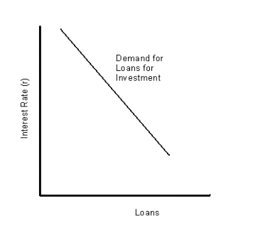
In sum, investment demand is a downward sloping function of the interest rate. The less it costs to borrow, the more attractive an investment opportunity becomes. Graphically, the demand for investment funds is, as shown in Figure 5-1, a downward sloping function of the interest rate.

Figure 5-1
Demand for loans

The demand for loans has an inverse relationship with the interest rate. As the real interest rate falls more projects are profitable to undertake

Saving

We now want to discuss the consumer’s saving and consumption decision. Saving is, after all income minus taxes minus consumption. Thus

S = Y – T – C.

That is,

Saving = Income less Taxes less Consumption

Motives for Saving

People save so that they can consume more in the future. A decision to spend now or save is really a choice of when to spend – now or in the future. The decision depends on wealth, disposable income, real interest rates and tastes or preferences for spending now versus waiting. While we will not engage in a complete discussion of the determinants of saving, the following examples will make some of the points.

· Fred and Barney have the same income this year. They are alike in all respect except that Fred gets a big inheritance from his beloved Aunt Matilida this year. Who is likely to save more from this year's income, Fred or Barney? Answer: Fred has more assets that Barney, and can live better. He is likely to spread his largess over several years, meaning that Fred will spend more this year than Barney. In turn, this means less saving this year.

· Fred and Barney have the same income this year. They are alike in all respect except that Barney has a generous pension plan. Fred has none. Who is likely to save more from this year's income, Fred or Barney? Answer: a true measure of assets includes funds in things like pension plans, not just in stocks, bonds and bank accounts. The logic given above applies here, so that Barney is likely to spend more this year than Fred. In turn, this means that Barney will save less this year.

· Fred and Barney have the same income this year. They are alike in all respect except that Barney has just made a killing in the stock market. Fred kept his money in Certificates of Deposit. Who is likely to save more from this year's income, Fred or Barney? Answer: look at the two questions above. Barney will save less this year.

· Fred and Barney have the same income this year. They are alike in all respect except that Fred expects a big pay raise next year. Who is likely to save more from this year's income, Fred or Barney? Answer: just as people base their consumption on assets and income, so too do people base their consumption on current and future income. This means Fred will spend more and save less this year.

· Fred has twice Barney's income this year. Who is likely to save more from this year's income, Fred or Barney? Answer: we just don't have enough information to tell.

Warning required by the Economist-General:

· In an introductory course, our discussion of the determinants of consumption and saving is quite simple. However, all of the examples given above have answers consistent with the more general theory of consumption. We return to examples like these to discuss how taxes and deficits affect saving and consumption.

The Role of Interest Rates

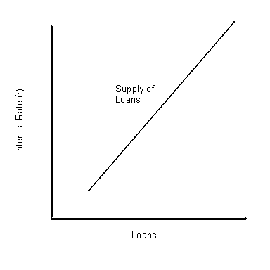
Without getting into a detailed discussion of the determinants of saving, common sense tells us that, the higher the interest rate, the more people will save. This guarantees us that the supply curve will be upward sloping, as shown in Figure 5-2. Of course, the examples we have given above indicate that this supply curve, like most supply curve has supply shifters.

Figure 5-2
Supply of loans

There is a direct relationship between the interest rate and the supply of loans

Equilibrium

We now come to the question of how saving and investment come into balance. The answer, of course, is the interest rate. As Figure 5-3 shows, the intersection of the supply and demand for loans determines the interest rate.

Figure 5-3
Equilibrium interest rate

S, I

r_o

Supply of Loans (Saving)

Demand for Loans (Investment)

The equilibrium interest rate is where the total demand for loans equals the total supply of loans.

Two Important Modifications

While the simple argument

Saving = Investment

captures the important point we want to make, there are two important modifications we must incorporate:

· The government almost never spends exactly what it takes in. In some years, it runs a deficit and borrows additional funds to cover its deficit; in yet other years, it runs a surplus and uses the funds to pay off its debts. In either case, government transactions affect the supply and demand for loans.

· In recent years, Americans have done substantial international borrowing and lending. International lending is around $300 billion per year, while international borrowing runs about $500 billion per year. We cannot neglect the international sector.

We take up each of these issues in turn.

Government Demand for Loans

To get the total demand for loans, we must add another component: the government’s demand for loans to cover its deficit. Note that this is the net demand of all governments, state, federal and local. In some years, this "demand" can be negative, as for example, when the government is paying down its debt. Some people argue that we should then treat the government surplus as a supply of loans. Nevertheless, there is a convention: we always treat the government's deficit as an addition, positive or negative, to the demand for loans.

Figure 5-5 illustrates the possibilities. Suppose the government is running a deficit. Then, as the upper left panel of Figure 5-5 shows, the total demand for loans shifts to the right. If the government is running a surplus, then there is a "negative demand for loans", also known as a surplus. The government's situation looks like the lower left panel of Figure 5-5 and the net effect, as the lower right panel shows, is to shift the demand for loans to the left.

Warning required by the Economist-General:

· Some people would like to argue that, when the government switches from a deficit to a surplus, it is now a supplier of loans instead of a demander. Instead, we should add the surplus to the supply of loans. Do not do that. This is just a convention. We always shift the demand for loans to adjust for the government's surplus or deficit. In any case, it makes no difference in our analysis.

· Why this convention? It is probably because, for most of the time since World War II, the Federal Government has run a deficit. Perhaps economists are creatures of habit.

	Figure 5-5 Total demand for loans
Deficit		Total Demand Investment Demand
Surplus		Investment Demand Total Demand
	A government deficit will cause a shift in the demand for total loans. If the government runs a deficit, total demand shifts to the right. If the government runs a surplus, total demand shifts to the left.

Let us illustrate the two cases. Figure 5-6 shows what will happen if the there is a government surplus. As you can see, the total demand curve lies to the left of the investment demand function. Thus the interest rate is lower than it would be without the deficit.

Figure 5-6
Equilibrium interest rate with Surplus

Funds from govt. Surplus

Funds from private saving

r_o

Total Demand

Investment Demand

Supply of Loans

The equilibrium interest rate is where the total demand for loans equals the total supply of loans. Here, the government surplus means that investment is greater than saving.

In the case of a government deficit, the demand curve will shift to the right. Investment will be less than saving. Table 5-7 shows how.

Figure 5-7
Equilibrium interest rate with Deficit

Private saving covering deficit

Private saving used for invest-ment

r_o

Investment Demand

Total Demand

Supply of Loans

The equilibrium interest rate is where the total demand for loans equals the total supply of loans. Here, the government deficit means that saving is greater than investment.

Warning required by the Economist-General:

· Be careful reading these two figures. Some people read them to say that when the government runs a deficit it "crowds out" investment, reducing the supply of saving for investment, and that, when it runs a surplus, it supplements private saving, making more available for investment. The truth is more complicated. Wait until the next lecture.

International Trade and the Loans Market

In discussing the loans market, we have treated it as solely a domestic one. Nevertheless, there is an important international aspect to this market. In 1998, for instance, Americans both borrowed and lent abroad, on net borrowing about $200 billion more than we lent.

Warning required by the Economist-General:

· An important qualification is being left out of this argument relating to exchange rate risk. We come back to this subject when we turn to the international sector.

Because there is an international capital market with an international interest rate, any difference between domestic demand and supply of loans is absorbed into the international market. If American demand for loans exceeds American Supply, we borrow the difference abroad; if American Supply exceeds American Demand, we lend abroad.

	Figure 5-8 Domestic and International Demand and Supply of Loans
rw	International Borrowing Domestic Demand for Loans Domestic Supply of Loans	World Demand for Loans World Supply of Loans
	The equilibrium interest rate is where the total demand for loans equals the total supply of loans. Here, the government deficit means that saving is greater than investment.

Figure 5-8 shows the equilibrium in this case, in both the domestic and the world market for funds. To make the graph simple, this graph only talks about the total demand for funds. It really doesn’t matter whether the demand for funds comes from the demand for investment or from a government deficit. As you can see from this graph, at the world interest rate – the rate that equates the world demand and supply of funds – there is a gap between the quantity of loans supplied and demanded domestically. International borrowing makes up this gap.

There is a lot of truth in this graph, but it is probably a little too simplistic. Americans probably face an upward sloping international supply curve of loans. The more we borrow, the higher the interest rate we pay. The more we lend abroad, the lower the interest rate we receive. Why? There is some preference to by everyone to lend domestically, where you know the market best. Thus, if Americans are borrowing abroad, they are probably paying a premium above the world interest rate.

Do changes in a country's supply and demand for loans affect the world rate? It depends. For a country such as Bolivia, the affect is probably negligible. Figure 5-9 shows what would happen with an increase in the Bolivia's demand for loans. There would be no change in the world rate, and Bolivia would simply borrow more from abroad.

	Figure 5-9 What Happens when Bolivia's Demand for Loans Increases
rw	DB International Borrowing Bolivian Demand for Loans Bolivian Supply of Loans	World Demand for Loans World Supply of Loans
	When Bolivia's demand for loans increases, there is no effect on the world interest rate. There is simply an increase DB in the amount being borrowed on international markets..
Warning required by the Economist-General:
· Saying that there is "no change" is a strong statement. A more precise statement would be that the change is negligible..

On the other hand, the United States is a major player in the world economy. When we increase our demand for loans, world rates will adjust. Figure 5-10 shows what would happen in this case.

	Figure 5-10 Impact of an American Increase in the Demand for Loans
Rw rw	International Borrowing American Demand for Loans American Supply of Loans	World Demand for Loans World Supply of Loans
	When the American demand for loans increases, the world demand shifts to the right. The world interest rate rises to Rw. There is both an increase in loans demanded and supplied in the United States. International borrowing may or may not increase.

Capital Flows and the Balance of Payments

At the beginning of this lecture, we stated:

We now turn to the subject of what determines the division of GDP between consumption and investment. In fact, we will go beyond Crusoe and include government borrowing and international trade in our discussion.

This condition is sometimes referred to as equilibrium in the goods market. That is, the demand and supply of GDP are equal.

In fact, what we have ended up with is Figure 5-8, showing equilibrium in the loans market. Rest assured that these are related. Whenever the loans market is in equilibrium, so too is the goods market. That is the total demand for goods and services will equal the supply of good and services.

To see why, note that equilibrium in the loans market requires that

S_domestic + S_foreign = I + DEF

where

· S_domestic = Domestic Saving

· S_foreign = Foreign Saving (Loans from Abroad)

· I = Investment

· DEF = Government Deficit

Obviously, the government deficit is equal to the difference between government purchases (G) and taxes (T), so we can rewrite our equation as

S_domestic + S_foreign = I +(G- T)

As to foreign saving, the only way foreigners can make investments in a country is by exporting more to that country than they import. Thus we know that

S_foreign = M- X

where

· M = Imports

· X = Exports

It is traditional to multiply this equation through by –1 and rewrite it as

-S_foreign = -(M- X)

When we discuss the international sector, the left hand side of this equation represents the balance in the capital account. That is, the amount we borrowed (or if it is negative) the amount we lent abroad. The right hand side represents the balance in the current account, which is the extent to which our exports exceeded our imports. (In fact that is why we multiply through by –1. The left hand side is then the amount we lend abroad or, if negative, the amount we borrow abroad; the right hand side is the amount by which exports exceed imports.)

In any case, our basic equation becomes

S_domestic + M- X = I + G- T

Or, rearranging terms

S_domestic = I + G- T + X-M

Finally, we know domestic savings is defined as the difference between after tax income (Y-T) and consumption, or

S_domestic = (Y - T) - C

That is enough to tell us that

Y – T - C = I + G- T + X-M

We can then simplify this equation to obtain:

Y = C + I + G + (X-M)

In short, when the demand and supply of loans are in balance so too is the goods market.

A Numerical Example

A numerical example may help make this issue clear. Table 5-4 gives some hypothetical data on GDP

Table 5-4 Some Illustrative GDP Data
Series	Value
Gross Domestic Product	100
Consumption	60
Taxes	10
Government Purchases of Goods and Services	20
Investment	35

Given these data, domestic income is $100. If consumers spend $60 on consumption and $10 on taxes, their saving is $30. There are two demands for loans: $35 for investment and $10 to cover the government deficit. The difference can be covered by foreigners deciding to put $15 of their savings into the United States, either by purchasing government bonds, shares in American businesses, or the like. In short, the difference between the domestic supply and demand for loans will be covered by $15 of international capital flowing into this country.

We cannot stop there, for there is another problem. These data indicate domestic production of $100 and domestic expenditures of $115 ($60 on consumption, $20 on government purchases of goods and services, and $35 of investment). Something has to give. What gives is that we must have net imports of $15 of goods and services.

Think about the patrons of Miller's Pizzeria consuming 115 pizzas while the Pizzeria bakes 100. To make this happen Miller's Pizzeria must send out to Dominos or Papa Johns for another 15 pizzas. They would have to import. So too it is with the country. We can no more spend $115 domestically while we are producing only $100 without net imports of $15.

It is no accident that the amount of net imports is exactly equal to the net capital flows. They must be equal. That is,

The Balance on Capital Account = Balance on Current Account

Essentially, having an international economy provides a third source of funds for the loan market (and one that can easily be positive or negative). We will return to this equation later in the course when we discuss the importance of capital flows.

This gets controversial. Many people, seeing net imports of $15 will cry that the nation is living beyond its means. We turn to this subject in depth later. For the moment, think of the following situation:

You are the manager of Miller's Pizzeria. Customers are ordering 115 pizzas, when you can only make 100. Would you not be better off importing 15 additional pizzas (perhaps discretely removing the Dominos boxes) and making the profit on 15 extra sales than refusing to "live beyond your means? Would we as a nation be better off reducing our investment by $15 to ensure we were not living beyond our means?

Real and Nominal Interest Rates

This is a good place to straighten out a major source of confusion between real and nominal interest rates. Most of the interest rates that you see discussed in places like the Wall Street Journal or TV newscasts are nominal interest rates that give the return in terms of the pictures of George Washington. That is, you lend me 100 pictures of George and I will return you (say) 106 pictures. (r_N = 6%) a year from now. The interest rates that banks quote for a loan or that you pay on your credit card are nominal interest rates.

Warning required by the Economist-General:

· This is not a trivial point. The distinction between real and nominal interest rates is vital. Indeed, one study suggested that the distinction between real and nominal rates is the key point for any macroeconomics course to get across.

Seeing how much you really earn

Economists talk about real interest rates, which give the return in terms of purchasing power. In other words, you lend me enough to purchase 100 pizzas and I will return you (say) enough to purchase 103 pizzas. (r_R = 3%)

An example will illustrate the relationship between the two. Last year, I lent you $100, which you promised to pay back a year from now plus 6% nominal interest. That is, you promised to give me back 106 pictures of George. Last year, pizza slices were selling for $2 (at least for the purpose of the example). I gave you the ability - and gave up the ability for myself - to purchase $100/$2 = 50 pizza slices. When you pay me back, I get $106, and I have earned a nominal return of 6%. My real return is measured in terms of the percent increase (decrease) in the number of pizza slices I can purchase.

Table 5-5 The Concept of Real and Nominal Rates Illustrated with Pizza Slices
Amount paid back	$106	$106	$106	$106
Increase in price of a slice of pizza	-2%	0	2%	4%
Price of a pizza slice	$1.96	$2.00	$2.04	$2.08
Number of pizza slices I can buy	54.1	53	52	51
Percent increase	8.2%	6.0%	3.9%	1.9%

There is a simple relation between the nominal interest rate (here, six percent) and the realized rate. As an approximation, subtract the inflation rate from the nominal interest rate. (If the inflation rate is negative, remember how to subtract a negative number). When you do, you will get the real return. (Or actually, you will get very close to it. There is a minor adjustment that you must apply to get the exact result, but it is not worth going into).

We summarize these relations between real and nominal returns with a simple relation, the so-called Fisher Equation.

· The realized real rate is given by

r_R @ r_N - p

where

r_R = real interest rate

r_N = nominal interest rate

p = Inflation rate

We can also use the equation to set future interest rates. To see how, suppose you want to borrow $100. To do so, I must give up 50 pizza slices (resetting their price to $2). The terms for lending depend on several factors:

Your credit worthiness

Tax considerations

My impatience motive

Inflationary Expectations

(We cross out the first two, because they will distract us here).

Suppose that I would want a reward of another three pizza slices for postponing consumption. That is, if I give up the right to consume 50 pizza slices today, I expect to consume 53 a year from now, I need a real return of 6%. I now want to know much inflation will occur over the next year.

Table 5-6 Forward-Looking Real and Nominal Rate Calculations Illustrated with Pizza Slices
If I expect an inflation rate of	-2%	0	2%	4%
The cost of a slice of pizza a year hence will be	$1.94	$2.00	$2.04	$2.08
And the cost of 53 pizza slices will be	$103.88	$106.00	$108.12	$110.24
The implied nominal interest rate is	3.9%	6.0%	8.1%	10.2%

In short, we can use the Fisher equation to set a nominal rate to get our desired real rate. We get another basic rule.

· Expected real rates and nominal rates are then related by a variant of the Fisher Equation

r_N @ r^e_R + p_e

where

r^e_R = Expected Real Rate

p^e = The expected inflation rate

Warning required by the Economist-General: · The Fisher Equation is fundamental. All Economists and All Economics students are required to learn and use the following relations between real and nominal interest rates.
Symbol	Meaning
p	The inflation rate
p^e	The expected inflation rate
rN	The nominal interest rate
rR	The realized real rate
r^eR	The expected real rate

Which Rate Matters?

It would be nice if all questions in economics were this simple. Where saving and investment are concerned, always use the real rate.

· If you are thinking of whether you should consume or save, you want to use the expected real rate. You want to know how many extra pizza slices you will get from dieting today.

· If you are thinking of investing, you still want to use the real rate. Here, you want to know how many slices of pizza you must sell in the years to come to pay back your investment.

There are cases where the nominal rate matters:

· If you are deciding many pictures of George Washington to carry in your pocket, the nominal rate matters. We will turn to this issue later.

· For some international exchange transactions, the nominal rate is the one that matters.

Warning required by the Economist-General:

· During the course of this semester, both the newspapers and the evening newscasts will probably carry a story describing how the Federal Reserve System is thinking about raising or lowering interest rates. If this story does not make it this semester, they will certainly carry one or more stories about how the Federal Reserve System should change interest rates, or might change interest rates, or recently changed interest rates.

· Do not believe everything you read or hear. As this lecture makes clear, the fundamental mechanism for setting interest rates is the process of equating Saving and Investment, with appropriate adjustment for Government deficits and the international sector. The Federal Reserve System does not set interest rates.

· There is a qualification. When we talk about the money supply, we will learn that the Federal Reserve System has limited control over one interest rate, called the Federal Funds Rate. However, we are getting ahead of our story.

Calculating Real and Nominal Rates

Most public discussions of interest rates focus on nominal interest rates, inasmuch as most loans are set in nominal terms. However, there are some government bonds which pay interest in real terms. In the late 1990's the Federal Government issued a series of Inflation Indexed Treasury Securities. These securities pay interest, but the redemption value is adjusted up for changes in the inflation rate. That is, though they pay off in pictures of George Washington, the number of pictures of George will be increased to keep the number of slices of pizza it purchases constant. The prices are given daily in Financial Newspapers.

For example, the June 28, 2000 issue of the Wall Street Journal quoted the data in Table 5-6 on Inflation Adjusted Securities:

Look, for instance at the first security. It pays a promised rate of 3.635%, matures in July 2002, and can be sold for 97 7/32 % of par and bought for 97 8/32% of par. (Par value is often set at $1,000). Because it sells at a small discount, the effective yield to maturity is 4.008%. Because of inflation to date, the government is obligated to pay $1,069 at maturity, not the $1,000 purchase price.

Table 5-6 Interest Rate Quotes on Inflation Adjusted Securities
Rate	Maturity	Bid/Asked	Yield	Accrued Principal
3.625	07/02	99-07/08	4.008	1069
3.375	01/07	95-28/29	4.093	1081

Because these securities are in real terms, the interest rates are the real interest rate. Thus, if you want to know the real rate between now and July 2002 it is 4.008%.

The same issue of the Wall Street Journal contained quotes on nominal securities. For example, a Treasury bond maturing in July 2002 has a nominal interest rate of 6.48%. Thus, as of June 20, 2000, the expected inflation rate for the next two years was

6.48% - 4.008% @ 2.47%

Warning required by the Economist-General:

· View this precise calculation cautiously. Different Treasury Securities have different tax provisions, as well as other provisions such as "call protection". Adjustment for these differences is quite complicated and well beyond this course. Nevertheless, this calculation does give the flavor of the use of real and nominal interest rates.

A Summing Up

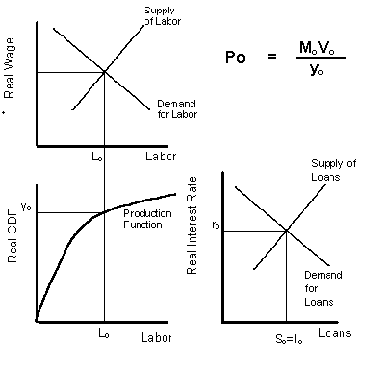
We can now summarize our model, with the aid of Figure 5-5, given below. This graph repeats what we have been studying in this lecture and the last. Starting with the upper left-hand panel, the demand and supply of labor sets the wage rate and the number of people working. Moving counterclockwise to the next panel, the combination of the number of people working and the production function determines real output, or real GDP. The supply and demand for loans, or, if you will, the supply of saving and the demand for investment funds determine the real interest rate. Of course, once we know the level of saving and investment, we know how much of GDP goes to consumption and how much goes to investment. Finally, the equation of exchange determines the price level.

There is a lot we want to do with this model during this course. In part, there are several "bells and whistles" we need to add to the model. We want to say something about how the money supply is determined, for instance. Our emphasis on long run and short run labor supply curves at the beginning suggest something else we want to add to the model, and we have not yet begun to discuss the role of the government in the economy. There is also a lot of material about the international sector to add to the model.

Figure 5-5
Our Basic Model

This figure summarizes the basic macroeconomic model. Starting with the upper left-hand panel and moving counterclockwise, the demand and supply of labor determines the number of people working. In turn, the number of people working determines the total level of GDP. The demand and supply of loans determines the real interest rate, and hence the division of output between consumption and saving. Finally, the equation of exchange determines the price level.

Relation to the Text

Each lecture ends with a section relating it to the text. In some cases, material is omitted, either because the text covers it well enough or because it is not worth learning. In other cases, material is added. Each of these “lectures” will end with a brief note relating the lecture to the text, describing what material is left to the student to learn alone and what material may safely be skipped.

Which Chapters does this lecture cover?

Section from Stockman	Coverage
Ch. 7, Interest Rates and Loan-Market Equilibrium	Covered
Ch. 7, Savings and the Supply of Loans	Covered
Ch. 7, Real and Nominal Interest Rates	Covered
Ch. 7, Summary of the Basic Model	Covered

What material is new?

The topics are the same. The examples comparing Fred's and Barney's saving behavior are added. We will build on them later.

©2000 by Greg Chase and Charles W. Upton. If you enrolled in Principles of Macroeconomics at Kent State University, you may print out one copy for use in class. All other rights are reserved.