Introduction to bivariate
statistics
Bivariate Association
Some Terms
Variance and
Covariance
The linear correlation
coefficient, r
So far, we have learned how the mean and standard deviation can be used to summarize data (data reduction). We have also learned how the central limits theorem and information about a known population distribution can be used to tests hypotheses about observational data. The z-tests and the t-tests enable us to infer information about the true, underlying population parameters from the observational samples we have collected.
All of these concepts are univariate applications, which means they are applied to the study of only one variable at a time. Using these methods we have touched on the concepts of data reduction and inference, two of the three primary reasons for which statistics are used. Association of variables, the third primary use for statistics, by definition, requires bivariate or multivariate data. To infer an association requires more than one variable. As we begin to discuss statistical association, you'll find that many of the univariate statistics we have learned will serve as building blocks for more complex statistics.
In many real world studies, we are interested in
how two or more variables measured on our sample object or
samples are related. Qualitatively, we may say that two
variables are similar, behave similarly, are associated,
related, or interdependent. These qualitative terms all imply
that there is some relationship between the two variables.
The following terms have specific statistical meaning. Try to
avoid using them unless you have that particular meaning in
mind: covariance,
correlation, orthogonal and non-orthogonal.
We'll discuss orthogonal and non-orthogonal in more detail later
in the multivariate section of the class. Note that statistical correlation is not the same as stratigraphic
correlation. In statistical
correlation, we will develop specific quantitative relationships
to describe bivariate associations. In stratigraphic
correlation, we match stratigraphic informatrion from diferent
locations to qualitatively determine if they are linked to the
same formation.
For now, let's start discussing the relationship
between variance, covariance and correlation.
There are many type of research questions that require us to understand the relationship between two variables. We can quantify this by determining the nature of their bivariate association. We might want to study how rainfall in a catchment basin is related to regional streamflow. Or we might want to study the relationship between some measure of soil quality and crop yield. Or we might want to know how large-scale climate processes such as the El Nino-Southern Oscillation (ENSO) affect temperature and precipitation in remote regions of the globe. In a paleoceanographic study, we may be interested in one variable, (e.g. the phosphate content of an ancient ocean), but may only be able to measure a related or proxy variable, such as the Cd content of shells from fossil benthic foraminifera.
In principle, there are two way we could approach these topics. We could seek to conduct controlled experiments in which we manipulated the value of one variable, and observe the effect on the other variable. Methods like this can be used to test relationships between soil quality and crop yield for example. This approach is ideal, because it provides a means of determining cause and effect. Unfortunately, we often lack the ability to conduct controlled experiments. This is particularly true in the earth sciences where controlled experiments are often impractical due to the spatial or temporal scales of the processes in question. In such cases, covariance or correlational methods can be applied to observational data to explore the bivariate relationships between two variables.
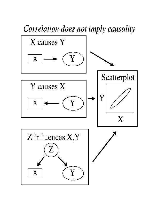
But it is important to keep in mind that we
cannot determine cause and effect from a correlational
study. Repeat after me: "Correlation does not imply
causality." Say this three times and commit it to memory!
Correlations tell us how two variables are related, but we learn
nothing about which of them (if either) may be causing the
relationship. Without an experimental manipulation we can't tell
which of the two variables is driving the relationship, or even
if there is some third variable that is the underlying cause.
This is illustrated in the following diagram.
Notice that the three relationships that are illustrated are
very different, but they all produce the same scatter plot and
have the same correlation value.
Here are some terms related to covariance and correlation analysis that are important to understand.
Reasons to use correlation:
Description - by learning how two
variables are related in a quantitative way we
learn something about the processes that relate
them.
Common variance - Variables that
are correlated, covary. We measure this through
covariance.
We will learn how to determine how much
of the variance in one variable in explained by its
correlation to another variable. As
pointed out in the text, this concept is related to prediction.
Prediction - If a correlation is
strong enough, we may be able to use it as a predictive
statistical tool. This concept will be very clear
when we consider the relationship between
correlation and least squares regression.
Ways to describe a correlation:
Linear vs. Non-Linear
- a scatter plot of two linearly correlated variables will
follow a
straight line with variable degrees of noise. In
contrast, if two variables follow some
arbitrary function they exhibit a non-linear
correlation.
Positive vs. negative - If
high values of one variable occur in conjunction with high
values
of another variable they are positively
correlated. If high values on one variable occur with
low values of another, they are said to be negatively
or inversely correlated.
Orthogonal - two variables that are unrelated or uncorrelated are said to be orthogonal.
Non-orthogonal - two variables that
are related or correlated are said to be non-orthogonal
Strong vs. weak - if much of the variability is explained or shared
between two variables,
they are said to have a strong correlation. Weak correlations
occur between variables that share
little common variance.
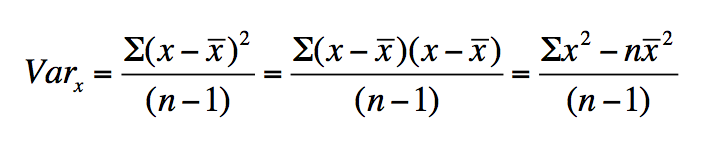
Earlier, we leared that we can measure the variability about the
mean of a distribution by calculating its variance:
The unbiased variance is the adjusted average of the sum of
least-squared deviations for each observation relative to the
sample average. As can be seen above, we can write this in a
number of ways. The first method above is the direct definition.
The definition at the right is easier to calculate using a
calculator. The middle definition helps us to undertstand
the relationship between variance and covariance. If two variables
share variance in common, they are said to covary. We can measure
the amount of information that is shared in common by calculating
their covariance. We can define this specifically in the following
way:
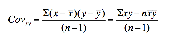
If we start with the middle defition
for variance that we just considered and substitute the
deviation of the y values from their sample average, we obtain
the reationship for the covariance of xy. Notice that the units
of covariance are the product of the units of the two variables,
xy. If two variables are unrelated, their covariance will be
zero. If two variables share common variance, then their
covariance will be non-zero. This formula should look similar,
as we have seen its "building blocks" previously. The covariance
is the average of the sum of cross products of the deviations of
x and y relative to their respective means. Because covariance
is a cross product of the two variables with difference
variances, the value can become very large. This can make it
difficult to compare the covariance between variables with very
different variances, but it does have the advantage of
preserving information about the original units of
measure. We can, however, scale the covariance so that we
can easily compare the covariance of variables with very
different units. We call the scaled covariance, the correlation
coefficent.
There are a number of ways that have been devised to quantify the correlation between two variables. We will be primarily concerned with the sample linear correlation coefficient. This is the scaled version of the covariance relatiation that we discussed above. This statistic is also referred to as the product moment correlation coefficient, or as Pearson's correlation coefficient. For simplicity, we will refer to it as the correlation coefficient. The sample correlation coefficient is denoted with the letter r, the true population correlation is denoted with the greek symbol, rho.
The linear correlation coefficient is defined as:
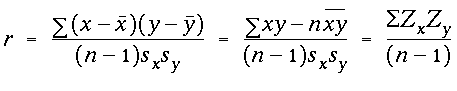
Notice that the correlation coefficient is
obtained from the covariance by dividing the covariance by the
product of the standard deviations of x and y, SxSy.
The associated degrees of freedom for the linear correlation coefficient is df = n-2 because we must know two mean values to calculate it.
There are two primary assumptions behind the use of the linear correlation coefficient:
(1) The variables must be related in a linear
way.
(2) The variables must both be normal in
distribution.
In fact, for the two variables to be correlated, they must exhibit a bivariate normal distribution. This second constraint makes sense when you consider the third way that r is written out above. It states that the r value is equal to the sum of the product of the observed z-scores for the variables x and y, normalized by n-1 observations. (This is also where the term product moment correlation coefficient arises - The mean is referred to as the first product moment, and the z-scores relate each observation to the mean.)
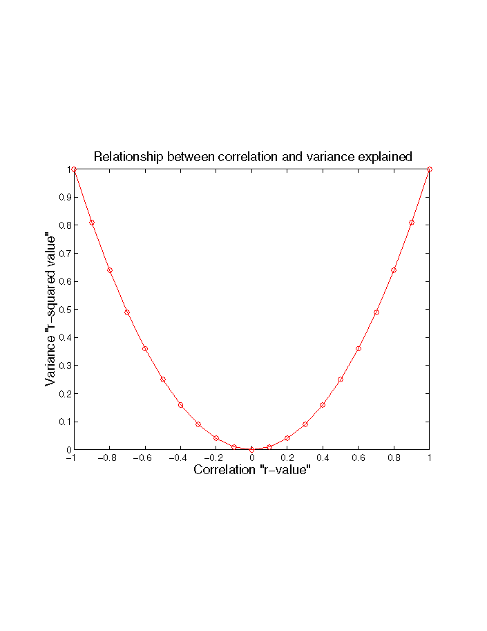
If we take the square of r, we obtain a measure of the amount of variance in x and y that is shared or common, which is called the coefficient of determination.
The relationship between r and r^2 is demonstrated by this plot.